목표
1. Argo 선택
2. Argo 데이터 다운로드
3. Argo 데이터 처리
Argo 선택
1. https://fleetmonitoring.euro-argo.eu/dashboard?Status=Active 접속
Argo Fleet Monitoring - Euro-Argo
fleetmonitoring.euro-argo.eu
2. 우측의 표시된 화살표를 클릭하여 지도 펼치기
(Argo 지점 로딩 시간이 걸릴 수 있습니다.)

3. 원하는 지점의 Argo 선택
4. 해당 Argo code 클릭

5. 해당 Argo 정보 확인

Argo 데이터 추출
1. https://data-argo.ifremer.fr/ 접속
Index of /
data-argo.ifremer.fr
2. dac/ 선택

3. 선택한 Argo와 같은 Data center 선택
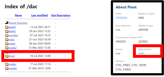
4. 선택한 Argo와 같은 code 선택

5. profiles/ 선택

6. 원하는 Cycle number를 선택하여 다운로드

코드 제작
|
clc; clear; close all;
addpath(genpath('../999__tool_box'))
%% input control
inp.code = 'D2901806';
inp.in = fullfile('01_data',inp.code);
inp.save = '02_save';
inp.fig = '03_figure';
if ~isfolder(inp.save)
mkdir(inp.save)
mkdir(inp.fig)
end
%% read & process
f.list = dir(fullfile(inp.in,'/*.nc'));
f.name = char(f.list.name);
for ii = 1:length(f.list)
route = fullfile(inp.in,f.name(ii,:));
n.info = ncinfo(route).Variables;
n.cycle = ncread(route,'CYCLE_NUMBER');
n.juld = ncread(route,'JULD',1,1); % 기준 : 1950-01-01
tp.id = sprintf('cyc_%03d',n.cycle);
d.(tp.id).time = datetime(n.juld+datenum(1950,1,1),'ConvertFrom','datenum');
d.(tp.id).cyc = n.cycle;
d.(tp.id).lon = ncread(route,'LONGITUDE',1,1);
d.(tp.id).lat = ncread(route,'LATITUDE',1,1);
tp.data_length = length(ncread(route,'PRES'));
d.(tp.id).dep = ncread(route,'PRES',[1 1],[tp.data_length 1]);
d.(tp.id).sal = ncread(route,'PSAL',[1 1],[tp.data_length 1]);
d.(tp.id).temp = ncread(route,'TEMP',[1 1],[tp.data_length 1]);
frame = 0:10:1000;
all.cyc(ii,1) = d.(tp.id).cyc;
all.sal(:,ii) = interp1(d.(tp.id).dep,d.(tp.id).sal,frame');
all.temp(:,ii) = interp1(d.(tp.id).dep,d.(tp.id).temp,frame');
end
save(fullfile(inp.save,[inp.code,'.mat']),'-struct','d')
%% figure control
fig.cyc_list = fieldnames(d);
for ii = 1:length(fig.cyc_list)
id = sprintf('%s',fig.cyc_list{ii});
fig.lon(ii) = d.(id).lon;
fig.lat(ii) = d.(id).lat;
fig.date{ii,1} = [datestr(d.(id).time,'yyyy-mm-dd'),' (',fig.cyc_list{ii}(end-2:end),')'];
end
tp.x = 32:.1:39;
tp.y = 0:.1:33;
for ii = 1:length(tp.x)
for jj = 1:length(tp.y)
fig.z(jj,ii) = sw_dens(tp.x(ii),tp.y(jj),0)-1000;
end
end
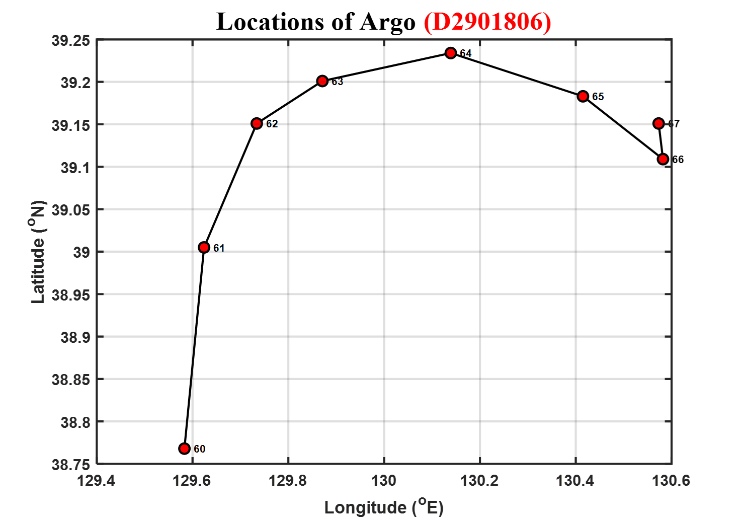
%% figure_location
figure('Visible','off')
set(gca,'fontname','time new roman','fontweight','bold','fontsize',15,'Box','on','linewidth',2,'Layer','top');
set(gcf,'color','w','Units','Normalized','OuterPosition',[0.1 0.2 .5 .7]);
hold on; grid on;
% plot
plot(fig.lon,fig.lat,'-ok','LineWidth',2,'MarkerSize',10,'MarkerFaceColor','r')
text(fig.lon+.02,fig.lat,num2str(all.cyc),'FontSize',10,'FontWeight','bold')
% deco
xlabel('Longitude (^oE)')
ylabel('Latitude (^oN)')
title(['Locations of Argo {\color{red}(',inp.code,')}'],'FontSize',25,'FontWeight','bold','FontName','times new roman')
%% figure_sal&temp
figure('Visible','off')
set(gcf,'color','w','Units','Normalized','OuterPosition',[0.1 0.2 .5 .7]);
subplot(1,2,1)
% set
set(gca,'fontname','time new roman','fontweight','bold','fontsize',15,'Box','on','linewidth',2,'Layer','top','YDir','reverse','XAxisLocation','top');
hold on; grid on;
% plot
for ii = 1:length(fig.cyc_list)
id = sprintf('%s',fig.cyc_list{ii});
plot(d.(id).sal,d.(id).dep)
end
% deco
xlabel('Salinity (psu)')
ylabel('Pressure (dbar)')
subplot(1,2,2)
% set
set(gca,'fontname','time new roman','fontweight','bold','fontsize',15,'Box','on','linewidth',2,'Layer','top','YDir','reverse','XAxisLocation','top');
hold on; grid on;
% plot
for ii = 1:length(fig.cyc_list)
id = sprintf('%s',fig.cyc_list{ii});
plot(d.(id).temp,d.(id).dep)
end
% deco
xlabel('Temperature (^oC)')
l = legend([fig.date],'Location','southeast');
set(l.Title,'String','Date (Cycle)')
sgtitle(['Argo {\color{red}(',inp.code,')}'],'fontsize',20,'fontweight','bold')
%% figure_contour
figure('Visible','off')
% set
set(gca,'fontname','time new roman','fontweight','bold','fontsize',15,'Box','on','linewidth',2,'Layer','top','YDir','reverse');
set(gcf,'color','w','Units','Normalized','OuterPosition',[0.1 0.2 .5 .7]);
hold on; grid on;
% plot
contourf(all.cyc,frame,all.sal)
% deco
ylim([0 810])
xlabel('Cycle number')
ylabel('Pressure (dbar)')
title(['Argo {\color{red}(',inp.code,')}'],'FontSize',25,'FontWeight','bold','FontName','times new roman')
% clolorbar
c = colorbar;
c.Label.String = 'Salinity (psu)';
c.Label.FontSize = 15;
colormap(jet(100))
figure('Visible','off')
% set
set(gca,'fontname','time new roman','fontweight','bold','fontsize',15,'Box','on','linewidth',2,'Layer','top','YDir','reverse');
set(gcf,'color','w','Units','Normalized','OuterPosition',[0.1 0.2 .5 .7]);
hold on; grid on;
% plot
contourf(all.cyc,frame,all.temp)
% deco
ylim([0 810])
xlabel('Cycle number')
ylabel('Pressure (dbar)')
title(['Argo {\color{red}(',inp.code,')}'],'FontSize',25,'FontWeight','bold','FontName','times new roman')
% clolorbar
c = colorbar;
c.Label.String = 'Temperature (^oC)';
c.Label.FontSize = 15;
colormap(jet(100))
%% figure_TS diagram
figure('Visible','off')
% set
set(gca,'fontname','time new roman','fontweight','bold','fontsize',15,'Box','on','linewidth',2,'Layer','top');
set(gcf,'color','w','Units','Normalized','OuterPosition',[0.1 0.2 .5 .7]);
hold on;
% plot
for ii = 1:length(fig.cyc_list)
id = sprintf('%s',fig.cyc_list{ii});
plot(d.(id).sal,d.(id).temp,'.','MarkerSize',10)
end
[c,h] = contour(fig.z,'LevelList',28:0.1:28.5);
clabel(c,h,'LabelSpacing',350)
% deco
xlim([32 38]);
ylim([0 33]);
xlabel('Salinity (psu)')
ylabel('Temperature (^oC)')
l = legend([fig.date],'Location','southeast');
set(l.Title,'String','Date (Cycle)')
title(['T-S diagram Argo {\color{red}(',inp.code,')}'],'FontSize',25,'FontWeight','bold','FontName','times new roman')
|


reference
1. https://www.youtube.com/watch?v=2vD6UDsW-GA
'데이터 처리' 카테고리의 다른 글
| [ 환경 자료 ] 국내 사이트 정리 (0) | 2023.08.08 |
|---|---|
| 국내 서해 utm 구역 경계 (0) | 2023.04.13 |
| [ KOHA ] 조위관측소 데이터 처리 (0) | 2023.04.09 |
| [ KOHA ] 국내 조위관측소 데이터 다운로드 (0) | 2023.03.31 |
| 조석 성분 분석 (0) | 2023.03.13 |